Polymer Chain Dynamics
The model of a polymer molecule used in this module consists of bead and springs forming a chain. The beads are hydrodynamics resistance sites that are dragged on by the suspending fluid. They also experience random Brownian forces caused by the thermal fluctuations in the fluid which are significant on the molecular scale. The spring is an entropic force pulling the adjacent beads together. In fact, the spring represents many monomer units that can coil and uncoil in response to the forces. This model is a reasonable representation of the polymer chain dynamics that actual polymer molecules undergo. By using a force balance which ignores the inertia effects, which have been shown to be small, and combining with a continuity statement, which guarantees that the chain configurations are conserved, a diffusion equation for the probability distribution function can be derived:
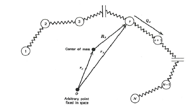
The position of each bead is given by , κ is the transpose of the velocity gradient tensor , ζ is the drag coefficient, N is the number of beads in the chain, k is Boltzmann’s constant, T is absolute temperature, and is the spring force. The probability distribution function gives the probability of finding the polymer chain in any given configuration as defined by the position vectors for the beads. For a chain of Hookean springs, the Rouse Model, the spring force on each bead is given by:
where the vectors are the connector vectors which point from bead to bead along the backbone of the chain. In order to consider non-linear springs we can replace each of the spring constants H by where is the square length of the bead-to-bead distance of the associated spring and b is an adjustable parameter to control the strength of the non-linear term.
In order to simulate the model above, the diffusion equation can be interpreted as an equivalent stochastic differential equation:
where is a random “white” noise process that can be simulated by a random number generator which produces a Gaussian distribution of zero mean and unit standard deviation. The equation above is integrated using a first-order Euler’s method to produce a trajectory of bead positions. The module gives a graphic representation of the result of this integration showing the polymer chain dynamics.